So, What are Algorithms? Algorithms, in computer science, are sets of steps for a computer program to achieve a goal. Depending on this "goal", we have a bunch of different algorithms. One such type of algorithm is the sort algorithm. A Sorting Algorithm is used to rearrange a given array or list of elements according to a comparison operator on the elements. These algorithms can have various procedures, creating the various sort algorithms we use today. A few of the most efficient algorithms are listed below :

QuickSort

First on the list, and most efficient, is the "QuickSort" Algorithm. QuickSort, is a Divide and Conquer algorithm, meaning that it selects an element as a pivot and consequently partitions the given array around the picked pivot. Now, how does QuickSort actually sort the array? Well, the first step would be to select a random element from the array, element x, which we'll consider the pivot. The algorithm first puts x at its correct position, then puts all the elements smaller than it before position x and similarly, puts all elements greater than it after position x.

There can be multiple ways to implement partition. The logic is quite straightforward, we start from the leftmost element, keeping track of the indexes of elements smaller than element x (our pivot element). While going through the array, if we find a smaller element, we swap that element with the element x. Otherwise, we ignore the current element and move to the next. Implementation of this method is provided below :

/* C++ implementation of QuickSort */
#include <bits/stdc++.h>

using namespace std;

// A utility function to swap two elements

void swap(int* a, int* b)

{
    int t = *a;
    *a = *b;
    *b = t;
}

/* This function takes the last element as a pivot, places
the pivot element at its correct position in sorted
array, and places all smaller (smaller than pivot)
to the left of the pivot and all greater elements to the right
of pivot */

int partition(int arr[], int low, int high)

{
    int pivot = arr[high]; // pivot
    int i
        = (low
           - 1); // Index of the smaller element and indicates
                 // the right position of pivot found so far

    for (int j = low; j <= high - 1; j++) {
        // If the current element is smaller than the pivot
        if (arr[j] < pivot) {
            i++; // increment index of the smaller element
            swap(&arr[i], &arr[j]);
        }
    }
    swap(&arr[i + 1], &arr[high]);
    return (i + 1);

}

/* The main function that implements QuickSort
arr[] --> Array to be sorted,
low --> Starting index,
high --> Ending index */

void quickSort(int arr[], int low, int high)
{
    if (low < high) {
        /* pi is partitioning index, arr[p] is now
        at the right place */

        int pi = partition(arr, low, high);

        // Separately sort elements before
        // partition and after partition

        quickSort(arr, low, pi - 1);
        quickSort(arr, pi + 1, high);

    }
}
/* Function to print an array */

void printArray(int arr[], int size)
{
    int i;
    for (i = 0; i < size; i++)
        cout << arr[i] << " ";
    cout << endl;

}

// Driver Code
int main()
{
    int arr[] = { 10, 7, 8, 9, 1, 5 };

    int n = sizeof(arr) / sizeof(arr[0]);

    quickSort(arr, 0, n - 1);

    cout << "Sorted array: \n";

    printArray(arr, n);

    return 0;

}

// This code is contributed by rathbhupendra (geeksforgeeks website)

Lomuto Partition ⬆️

Analysis of QuickSort :

The time taken by QuickSort in general can be written as follows :

T(n) = T(k) + T(n-k-1) + Θ(n)**

Worst Case Scenario - Θ(n²)
Best Case Scenario - Θ(nLogn)

Admittedly, the worst-case time compressibility of QuickSort, being Θ(n^2) is quite high. However, it is much quicker in practice as the worst-case scenario is rarely faced. QuickSort can be implemented in different ways by changing the choice of the pivot therefore, the worst case rarely occurs for a given type of data

---

Merge Sort

Merge sort, on the other hand, uses the "Divide and conquer" strategy. Diving an array into its consistent subarrays, It sorts these subarrays and then merges the subarrays together to form a completely sorted array.

Note: a "subarray" is just a fancy way of saying "a part of an array" or "a smaller section of an array".

What are the benefits of using Merge sort?
Merge sort is used to sort large arrays in meagre time. Another great thing about using merge sort is the fact that it is a stable sort. A stable sort is a sort that preserves the original order of the given array, which means that if it encounters two equal elements in the array, it will put the element that was first in the given array before the second equal element, therefore preserving the original sequence.

Working process :

Merge sort is basically an algorithm that continuously divides an array into smaller and smaller arrays until the array becomes empty or has only one element left.

For example, we're given an array consisting of 6 elements:

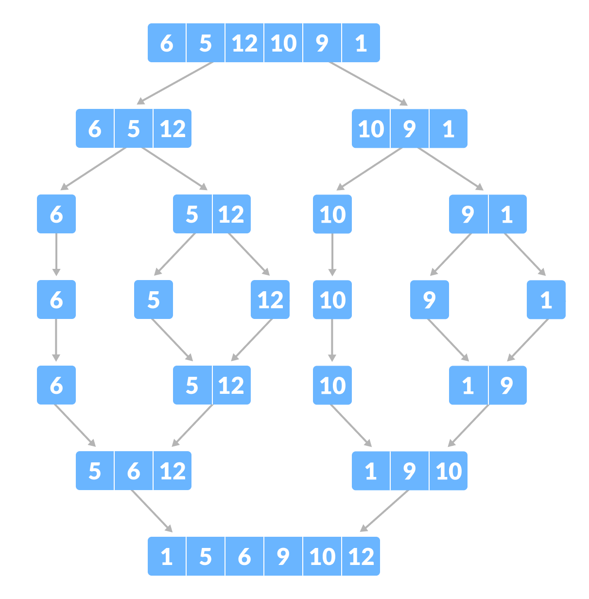
The first step that the merge sort algorithm would implement would be to break this array into equal halves. This algorithm works recursively meaning that it keeps on dividing the array until it cannot be divided further. Once all the subarrays are divided and sorted, they are merged together to form a completely sorted array.

The Algorithm for Merge Sort :

step 1: start

step 2: declare array and left, right, mid variable

step 3: perform the merge function.
if left > right
return
mid= (left+right)/2
mergesort(array, left, mid)
mergesort(array, mid+1, right)
merge(array, left, mid, right)

step 4: Stop

Implementation for Merge Sort :

# Python program for implementation of MergeSort
def mergeSort(arr):
    if len(arr) > 1:
         # Finding the mid of the array
        mid = len(arr)//2
        # splicing the list before the middle (therefore in case of an array     having an odd number of elements, the left halve gets more elements.

        L = arr[:mid]
        # splicing the list after the middle
        R = arr[mid:]
        # Sorting the first half by recursion
        mergeSort(L)
        # Sorting the second half by recursion
        mergeSort(R)
        i = j = k = 0

        # Copy data to temp arrays L[] and R[]
        while i < len(L) and j < len(R):
            if L[i] <= R[j]: #if the first element of the left halve is greater than the first element of the right halve
                arr[k] = L[i]
                i += 1
            else:
                arr[k] = R[j]
                j += 1
            k += 1

        # Checking if any element was left
        while i < len(L):
            arr[k] = L[i]
            i += 1
            k += 1

        while j < len(R):
            arr[k] = R[j]
            j += 1
            k += 1

# Code to print the list

def printList(arr):
    for i in range(len(arr)):
        print(arr[i], end=" ")
    print()

# Driver Code
if __name__ == '__main__':
    arr = [12, 11, 13, 5, 6, 7]
    print("Given array is", end="\n")
    printList(arr)
    mergeSort(arr)
    print("Sorted array is: ", end="\n")
    printList(arr)

# This code is contributed by Mayank Khanna (Geeks for Geeks website)

Time Complexity :

Best, Worst and Average cases: As merge sort divides the array into two halves, sorts them and then merges them together in linear time, the time complexity for all three cases is θ(nlogn).

---

Bubble Sort

Bubble Sort is the simplest sorting algorithm that works by repeatedly swapping the adjacent elements if they are in the wrong order (that is if the second element is smaller than the first). However, this algorithm is not suitable for large data sets as its average and worst-case time complexity is quite high.

Working :

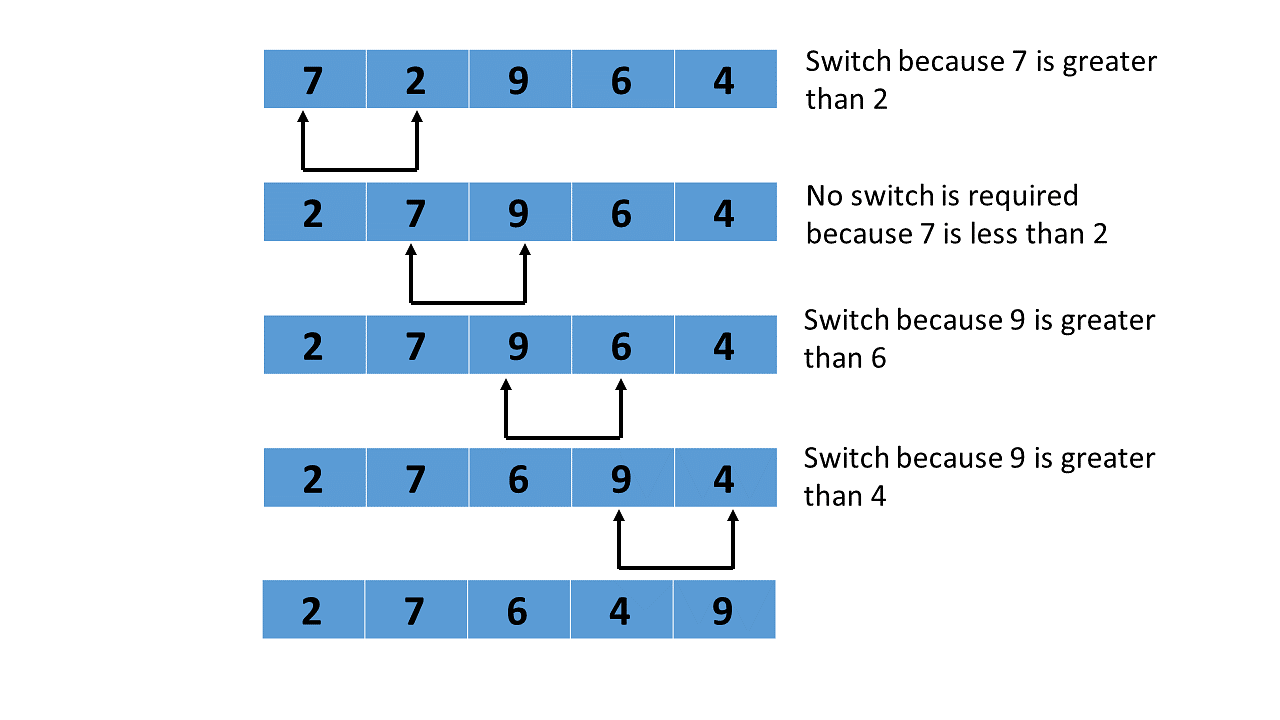
Bubble sort starts with the first element of the given array, which we call the 'bubble element. It then continues to swap that element with the adjacent elements if they are placed in the wrong order up until the end of the array. For example :

Algorithm for Bubble Sort :

begin BubbleSort(list)

   for all elements of list
      if list[i] > list[i+1]
         swap(list[i], list[i+1])
      end if
   end for

   return list

end BubbleSort

Implementation :

def bubbleSort(arr):
    n = len(arr)
    # Traverse through all array elements
    for i in range(n):
        # Last i elements are already in place
        for j in range(0, n-i-1):
            # traverse the array from 0 to n-i-1 (end of the array)
            # Swap if the element found is greater than the next element
            if arr[j] > arr[j+1]:
                arr[j], arr[j+1] = arr[j+1], arr[j]
# Driver code to test above
if __name__ == "__main__":
  arr = [5, 1, 4, 2, 8]
  bubbleSort(arr)
  print("Sorted array is:")
  for i in range(len(arr)):
      print("%d" % arr[i], end=" ")

Time Complexity :

Worst and Average case: The worst and average cases occur when the array is reverse-sorted.

Total number of comparison (Worst case) = n(n-1)/2*
Total number of swaps (Worst case) =* n(n-1)/2

Therefore, the time complexity is O(N²)*.*

Best Case: The best case for bubble sort is when the given array is already sorted. The time complexity for this is O(N)*.*

---

Selection Sort

The selection sort algorithm sorts an array by repeatedly finding the minimum element from the unsorted part and placing it at the front. ( Yes, at the beginning there is no "sorted part" so we traverse the entire array ).

Working :

For this example, consider array of n=5 to be arr[] = {48,52,13,34,19}

First Pass :
For the first pass in the selection sort algorithms, we traverse the array from index 0-4. As a result of this traversal (where we also simultaneously compare elements), we find that 13 is the lowest element. Replacing the element at index 0 (48) with 13,
The new array becomes - {13,52,48,34,19}

Second Pass :
For the second pass, the algorithm skips over the sorted element (which is the element at position 0) and iterates over the remaining unsorted portion. It finds the smallest number and then places it before the unsorted section (i.e. after element[0]).
The new array becomes - {13,19,48,34,52}

Third Pass :
For the third pass, the algorithm skips over the sorted elements (the elements at indexes 0 and 1) and iterates over the remaining unsorted position. It finds the smallest number from the unsorted portion and once again places it after the sorted portion and before the unsorted portion.
The new array becomes - {13,19,34,48,52}

Fourth pass :
For the fourth pass, the algorithm skips over the sorted elements (elements at indexes 0, 1 and 2) and iterates over the unsorted elements. Fortunately, this 'unsorted' portion is already sorted as 48 is placed before 52. And there we have our fully sorted array -
{13,19,34,48,52}

Implementation :

import sys
A = [64, 25, 12, 22, 11]
# Traverse through all array elements
for i in range(len(A)):
    # Find the minimum element in remaining
    # unsorted array
    min_idx = i
    for j in range(i+1, len(A)):
        if A[min_idx] > A[j]:
            min_idx = j   
    # Swap the found minimum element with
    # the first element       
    A[i], A[min_idx] = A[min_idx], A[i]

# Driver code to test above
print ("Sorted array")
for i in range(len(A)):
    print("%d" %A[i],end=" ")

Time Complexity :

In the selection sort algorithm, the time complexity is O(n²) in all three cases. This is because, in each step, we are required to find minimum elements so that they can be placed in the correct position. Once we trace the complete array, we will get our minimum element.

---

What is the time complexity of an algorithm? :

Instead of measuring the actual time required in executing each statement in the code, Time Complexity considers how many times each statement executes.

O(nlogn) > O(n²) > O(n)